Overhead lines
Electricity is carried around the country on overhead lines at various voltages. All overhead lines produce electric and magnetic fields. The fields are highest directly under the line and reduce rapidly as the distance from the line increases.
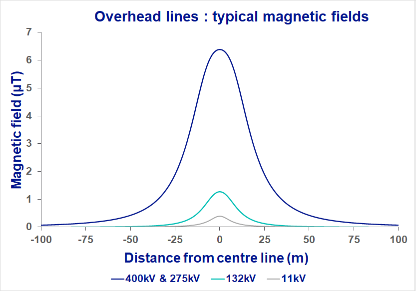
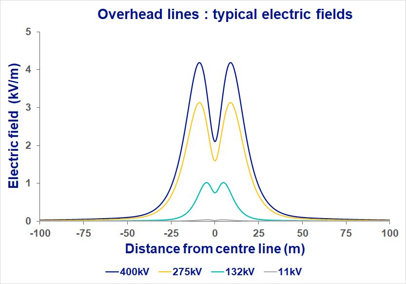
There are many factors that affect the EMFs that an overhead line produces but in general overhead lines of the same voltage will produce similar fields. Below are some graphs and a table of calculations of typical fields from different types of overhead line. As can be seen in the graphs below the fields are highest close to the line and then reduce with distance.
Typical UK ground-level fields from overhead power lines
| Magnetic field (µT) | Electric field (V) | ||
|---|---|---|---|
| The largest steel pylons (400 kV and 275 kV) |
Typical field (under line) Typical field (50 m to side) |
5 - 10 0.4 - 0.6 |
3,000 - 5,000 50 - 100 |
| Smaller steel pylons (132 kV) |
Typical field (under line) Typical field (50 m to side) |
0.5 - 2 0.03 - 0.2 |
500 - 3,000 20 - 100 |
| Medium wooden poles (11 kV) |
Typical field (under line) Typical field (50 m to side) |
0.4 - 1 0.01 - 0.03 |
50 - 200 1 - 5 |
| Smallest wooden poles (230 V) |
Typical field (under line) Typical field (50 m to side) |
0.05 - 0.2 <0.01 - 0.02 |
<1 <1 |
The electric and magnetic fields that are produced by overhead lines depend on a number of factors. The main factors for electric and magnetic fields are listed below:
Magnetic fields:
Current: The higher the current flowing the higher the magnetic field.
Clearance of wires to the ground: The higher the wires above the ground, the lower the electric field.
Phasing of the circuits: The way the that circuits are arranged on the pylon can impact the fields. See more here.
Electric fields:
Voltage: The higher the operating voltage of the overhead line the higher the electric field.
Size of the conductor bundle: Where there are more wires or conductors, this can increase the electric field.
Clearance of wires to the ground: The higher the wires above the ground, the lower the electric field.
We aim to give typical fields for different types of overhead lines, but the precise fields will differ according to the specific overhead line.